Most of this is from my class notes for the session - DSCI 6653 - Bayesian Data Analysis at the University of New Haven.
Bayesian optimization is a strategy for global optimization of black-box functions. In simpler terms, it is a smart way to find the best settings for a complex system where checking each setting is costly or time-consuming.
Instead of guessing randomly or checking a grid of points, it builds a probabilistic model of the function (often called a “surrogate”) to decide where to sample next.
This process relies on balancing two competing goals: Exploration (looking in places where we don’t know much yet) and Exploitation (refining our knowledge in areas that already look promising).
Step 1: The Intuition
Imagine you are a gold prospector on a vast, rugged piece of land. Your goal is to find the highest concentration of gold (the global maximum), but there is a catch:
Drilling is expensive: It costs a lot of money and time to set up a rig and drill a test hole. You can’t just drill everywhere.
Blind Search: You can’t see the gold from the surface. You only know how much gold is there after you drill.
This is exactly the problem Bayesian Optimization solves. It helps you decide where to drill next to get the best results with the fewest drills.
To make this decision, you use two main tools in your “mental map”:
The Surrogate Model (The Map): After every drill, you update your sketch of the terrain. If you found gold in one spot, you guess there might be more nearby. If you found nothing, you assume that area is barren. This sketch gives you a probability of finding gold across the map.
The Acquisition Function (The Strategy): This is the rule you use to pick the next spot. You have to balance two instincts:
Exploitation: Drilling near where you previously found gold. It’s a safer bet, but you might get stuck finding only small nuggets (a local maximum).
Exploration: Drilling in a completely empty part of the map. It’s risky (you might find nothing), but it’s the only way to find a massive vein of gold hidden in the unknown (the global maximum).
If you just stick to what you know (Pure Exploitation), you might be standing right next to a massive vein of gold (the global maximum) and never find it because you’re too busy digging up small nuggets elsewhere (local maximum).
So, the “Golden Rule” of Bayesian Optimization is that we need a strategy to balance these two:
Exploration: Checking the unknown.
Exploitation: Refining the known.
Step 2: The Mechanics
Now that we have the intuition, let’s look at the actual machinery that makes this work. In the math world, we don’t have a physical map or a gut feeling. We have two specific components:
The Surrogate Model (Gaussian Process): This acts as our probability map. It estimates what the function looks like based on the points we’ve already checked. It gives us a mean (expected value) and uncertainty (variance) for every point.
The Acquisition Function: This is the formula that decides where to sample next. It takes the “map” from the Surrogate Model and calculates a score for every possible point, balancing exploration and exploitation.
Let’s focus on the Surrogate Model first.
Imagine we have drilled two holes. One found a little gold, the other found none. We have no idea what is happening between those two holes.
If we want to build a model that guesses what the terrain looks like in the gaps, how confident should we be about our guess in the middle of those two distant points compared to a spot right next to a hole we already drilled? Less confident, right? he further we are from a drilled hole, the “fuzzier” our map becomes. We just don’t know what’s out there.
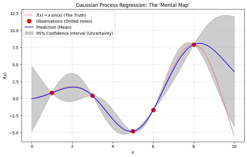
This is why the Gaussian Process (GP) is the standard tool here. For every single point on the map, it doesn’t just give us a single guess; it gives us a probability distribution (a bell curve).
This gives us two key pieces of data for every coordinate:
The Mean (\mu) : Our best guess for how much gold is there.
The Standard Deviation (\sigma) : Our uncertainty.
Note: Notice in the diagram how the shaded region (uncertainty) gets “pinched” tight near the black dots (data points) and balloons out in the empty spaces? That ballooning is the math telling us, “I have no idea what’s happening here!”
The Acquisition Function
Now we need a rule to look at that GP and say, “Drill here next.” This rule is the Acquisition Function.
A very common one is called Upper Confidence Bound (UCB). The formula looks roughly like this:
$$\text{Score} = \text{Mean} + (\kappa \times \text{Uncertainty})$$Mean: High predicted value (Exploitation)
Uncertainty: High potential to learn something new (Exploration)
(\kappa) (Kappa): A number we choose to tune our strategy.
If we set that (\kappa) (kappa) value to be very, very high, are we acting more like a safe, conservative miner, or a risky, adventurous explorer? We are acting like an adventurous explorer.
A high (\kappa) value boosts the “Uncertainty” part of the equation, meaning the algorithm is willing to ignore the safe bets (high Mean) to go check out the mysterious, unknown areas (high Uncertainty). It becomes an adventurous explorer.
So, the full Mechanics cycle looks like this:
Update Model: The Gaussian Process looks at the data we have so far.
Pick a Point: The Acquisition Function (like UCB) calculates the score for every point and picks the winner.
Evaluate: We actually “drill” at that spot (calculate the real result).
Repeat: We add that new data to our model and loop again.