Opening the Black Box: How to See What Your Vision Language Model is Actually Looking At

When a doctor examines a chest X-ray and says “I see signs of pneumonia in the lower right lung,” you can ask them to point at exactly what they’re seeing. They can circle the cloudy region, explain why it looks abnormal, and walk you through their reasoning. But when an AI system analyzes the same X-ray and reaches the same conclusion, what is it actually looking at? Is it focusing on the lung tissue, or has it learned some spurious shortcut, like the font used for the patient’s name?

This question sits at the heart of AI safety in medicine. If we’re going to trust AI systems to help with diagnostic decisions, we need to peer inside them and verify they’re looking at the right things for the right reasons.

In this post, I’ll explain a method called “Generic Attention-model Explainability” developed by Chefer, Gur, and Wolf that lets us generate visual explanations for what transformer-based AI models are paying attention to. We’ll build up the intuition piece by piece, starting from the basics and working toward the full algorithm. I’ve also implemented this method for Google’s MedGemma medical vision-language model, and I’ll share results showing the technique in action on real medical images.

My implementation: github.com/thedatasense/medgemma-explainer

Also you can open a notebook in Google colab that explains the concepts and a demo with the below link.

By the end, you’ll understand not just what the method does, but why it works.

Part 1: The Problem with Asking “What Did You See?”

Imagine you’re teaching a child to identify birds. You show them pictures, and they learn to say “that’s a robin” or “that’s a crow.” They get pretty good at it. But one day you notice something strange: they’re identifying robins correctly even in photos where the bird is tiny and blurry. How?

You investigate and discover they’ve learned a shortcut. Robins often appear in photos with green lawns in the background, while crows appear against gray skies. The child isn’t identifying birds at all. They’re identifying backgrounds.

This is exactly what can happen with AI systems. A famous example from medical imaging: researchers found that an AI trained to detect COVID-19 from chest X-rays had learned to recognize the font used by certain hospitals, which happened to correlate with COVID cases during the training period. The model worked great on test data from those hospitals, but it wasn’t actually learning anything about lungs.

The scary part? Without a way to see what the model is looking at, you’d never know. The accuracy numbers would look great right up until the model failed catastrophically on patients from a different hospital.

This is why explainability matters. We need to open up these models and see where their attention is directed.

Part 2: How Transformers Pay Attention

Before we can explain what a model is looking at, we need to understand how modern Vision Language models “look” at things in the first place. The key mechanism is called attention.

The Cocktail Party

Imagine you’re at a crowded party. Dozens of conversations are happening simultaneously, creating a wall of noise. Yet somehow, when someone across the room says your name, you hear it. Your brain has learned to selectively attend to relevant information while filtering out the rest.

Transformer models do something similar. When processing an image and a question like “Is there a fracture in this X-ray?”, the model doesn’t treat every pixel and every word as equally important. It learns to focus its computational resources on the parts that matter for answering the question.

Attention as a Spotlight

Think of attention as a spotlight that the model can shine on different parts of its input. When reading the word “fracture” in the question, the model might shine its spotlight on certain regions of the X-ray. When it encounters the word “bone” in its internal processing, the spotlight might shift to highlight skeletal structures.

Technically, attention works through a learned matching process. Each piece of input (called a “token”) asks a question: “What should I pay attention to?” This is called a query. Every other token offers up a description of itself, called a key. The attention mechanism computes how well each query matches each key, producing a set of attention weights that sum to one. High weights mean “pay close attention to this,” while low weights mean “mostly ignore this.”

Here’s the crucial insight: these attention weights create a map of relationships. If token A has high attention weight on token B, it means A is gathering information from B. By examining these weights, we can see what’s influencing what.

Multiple Heads, Multiple Perspectives

Modern transformers don’t use just one spotlight. They use many, called “attention heads.” Each head can focus on different aspects of the input. One head might track syntactic relationships (subject-verb connections in text), another might track semantic similarity (words with related meanings), and another might track positional relationships (things that are close together).

It’s like having a team of detectives investigating a case. One looks for physical evidence, another interviews witnesses, a third analyzes financial records. Each brings a different perspective, and the final conclusion synthesizes all their findings.

Layers Upon Layers

Transformers also stack multiple layers of attention. The first layer might capture simple relationships: “this word relates to that word.” But higher layers can capture more complex, abstract patterns: “this concept connects to that concept in this particular way.”

Think of it like the visual system in your brain. Early layers detect edges and colors. Middle layers combine those into shapes and textures. Higher layers recognize objects, faces, and scenes. Each layer builds on the representations from the layer below.

Part 3: The Challenge of Multi-Layer Attribution

Now we arrive at the core problem that Chefer et al. set out to solve.

If we want to know what the model looked at to produce its output, we can’t just examine the attention weights from a single layer. The information has been transformed, combined, and re-routed through dozens of layers. The final output is influenced by patterns that were established early and propagated forward, modified at each step.

The River Delta

Imagine tracing where a drop of water in the ocean came from. You find it at the river’s mouth, but that river was fed by dozens of branches of river, each of which was fed by smaller streams, each of which collected from countless tiny sources across a vast watershed.

The water at the mouth contains contributions from all those sources, but the contributions aren’t equal. A large tributary contributes more than a tiny stream. And some sources might have their water diverted or absorbed before it reaches the ocean.

This is exactly our situation with attention. The final output token is like the water at the river’s mouth. It contains information that flowed from all the input tokens (the sources), but that information passed through many intermediate stages (the tributaries), being combined and filtered at each step.

To understand where the output came from, we need to trace these flows backward through the entire network.

Why Raw Attention Fails

A naive approach is to just look at the attention weights in the final layer. After all, that’s the last step before the output, so shouldn’t it tell us what the model was looking at?

Unfortunately, no. The final layer’s attention operates on highly processed representations, not the original input. By that point, information from many different input tokens has been mixed together. When the final layer attends to position 47, it’s not attending to whatever was originally at position 47. It’s attending to a rich mixture of information that has accumulated at that position through all the previous layers.

It’s like asking “where did this river water come from?” and answering “from right there, just upstream.” Technically true, but it misses the entire watershed that actually supplied the water.

The Rollout Approach and Its Limitations

One early solution was called “attention rollout.” The idea is to multiply attention matrices from consecutive layers together, tracing how attention flows through the network.

If layer 1 says “token A attends to token B” and layer 2 says “token B attends to token C,” then we can infer that token A indirectly attends to token C through the path A→B→C. By multiplying attention matrices, we can compute these indirect attention relationships.

This is a step in the right direction, but it has a fundamental flaw: it treats all attention equally, whether positive or negative. In reality, some attention connections amplify information while others suppress it. When we multiply matrices together without considering these signs, positive and negative contributions can cancel out in misleading ways.

Imagine tracking money flow through a company. Some transfers add money to departments, others subtract it. If you just add up all the transfers without considering direction, you’ll get a very wrong picture of where resources actually ended up.

Part 4: The Chefer Method, Step by Step

Now we’re ready to understand the solution that Chefer et al. developed. Their method addresses the limitations we’ve discussed by carefully tracking how relevance propagates through the network while respecting the gradient information that tells us whether connections are helpful or harmful.

The Core Insight: Gradients Tell Us What Matters

Here’s a key insight: not all attention is created equal. When the model is deciding whether to output “yes” or “no” for “Is there a fracture?”, some attention connections are crucial to that decision while others are incidental.

How can we tell which is which? Gradients.

When we train neural networks, we compute gradients that tell us how changing each parameter would affect the output. But we can also compute gradients for intermediate values like attention weights. If changing an attention weight would significantly change the output, that weight has high gradient magnitude. If changing it would barely matter, the gradient is small.

By multiplying attention weights by their gradients, we can identify which connections actually matter for the specific output we’re trying to explain.

The Recipe

Let me walk through the algorithm step by step, building intuition as we go.

Step 1: Initialize with Identity

We start by creating a “relevance matrix” R that’s initially an identity matrix. An identity matrix has ones on the diagonal and zeros everywhere else. This represents our starting assumption: before any attention happens, each token is relevant only to itself.

Think of it as the starting state before the cocktail party begins. Everyone is self-contained, not yet influenced by anyone else.

Step 2: Process Each Layer

For each attention layer in the network, we update R to account for the new connections being made. The attention matrix A tells us how tokens attended to each other at this layer.

But we don’t use A directly. First, we weight it by the gradient to identify which connections matter:

Ā = average across heads of (gradient × attention)⁺

The × means element-wise multiplication. The ⁺ means we keep only positive values, setting negatives to zero. The average combines information from all the attention heads.

Why remove negatives? Because we’re tracking positive relevance, contributions that support the output. Negative gradients indicate connections that would hurt the output if strengthened, and we don’t want those polluting our relevance map.

Step 3: Accumulate Through Residual Connections

Modern transformers have “residual connections” that allow information to skip layers. This means the output of a layer is the sum of the attention output plus the original input, passed through unchanged.

To account for this, we add the new relevance to the existing relevance rather than replacing it:

R = R + Ā × R

The matrix multiplication Ā × R is the key operation. It says: “The relevance of token i to token j is the sum over all intermediate tokens k of how much i attends to k times how relevant k was to j.”

This is exactly the tributary logic. To know how much water source i contributes to outlet j, you sum over all intermediate points: how much flows from i to each intermediate point, times how much that point contributes to j.

Step 4: Extract the Explanation

After processing all layers, R contains the accumulated relevance. To explain a particular output token, we look at the row of R corresponding to that token. This row tells us how relevant each input token is to that output.

For image-text models, we can split this relevance vector into the image tokens and text tokens, giving us separate explanations for what visual regions and what words influenced the prediction.

A Worked Example

Let’s trace through a tiny example to make this concrete. Imagine a three-token sequence and a two-layer transformer.

We start with:

R = [1 0 0]
    [0 1 0]
    [0 0 1]

Each token is relevant only to itself.

Layer 1 has gradient-weighted attention:

Ā₁ = [0.1 0.3 0.2]
     [0.2 0.1 0.4]
     [0.3 0.2 0.1]

Token 0 attends mostly to token 1 (weight 0.3). Token 1 attends mostly to token 2 (weight 0.4). Token 2 attends mostly to token 0 (weight 0.3).

We update R:

R = R + Ā₁ × R
R = I + Ā₁ × I
R = I + Ā₁
R = [1.1 0.3 0.2]
    [0.2 1.1 0.4]
    [0.3 0.2 1.1]

Now token 0 has picked up some relevance from tokens 1 and 2. The diagonal values increased slightly because of self-attention.

Layer 2 has gradient-weighted attention:

Ā₂ = [0.2 0.4 0.1]
     [0.1 0.2 0.5]
     [0.4 0.1 0.2]

We update R again:

R = R + Ā₂ × R

I’ll spare you the matrix arithmetic, but the result is that R now captures both direct attention (token i attended to token j at some layer) and indirect attention (token i attended to token k, which had previously gathered information from token j).

If we want to explain what influenced token 2, we look at row 2 of the final R. If we want to explain token 0, we look at row 0.

Part 5: Applying This to Vision-Language Models

The method we’ve described works for any transformer. But applying it to vision-language models like MedGemma requires understanding how these models are structured.

How Images Become Tokens

Vision-language models convert images into sequences of tokens that can be processed alongside text. The typical approach uses a vision encoder that divides the image into patches (small rectangular regions) and produces one token per patch.

For MedGemma, an 896×896 pixel image is divided into 14×14 pixel patches, producing a 64×64 grid of patches. These are then pooled down to a 16×16 grid, yielding 256 image tokens. These 256 tokens capture the visual content of the image in a form the language model can process.

When you ask MedGemma “Is there a fracture in this X-ray?”, the model receives a sequence that looks like:

[img_0, img_1, ..., img_255, "Is", "there", "a", "fracture", "in", "this", "X", "-", "ray", "?"]

The first 256 positions are image tokens. The rest are text tokens. The model’s attention operates over this combined sequence, allowing image tokens to attend to text and vice versa.

Generating the Explanation

When we apply the Chefer method to this combined sequence, we get a relevance vector that tells us how much each position influenced the output. The first 256 values correspond to image regions. We can reshape these into a 16×16 grid and overlay it on the original image as a heatmap.

High values indicate “the model looked here when generating its answer.” Low values indicate “this region didn’t much matter.”

For the text tokens, we get relevance values that tell us which words in the question were most important. If the question was about fractures, we’d expect “fracture” and “bone” to have higher relevance than “is” or “there.”

Part 6: The Method in Action, My MedGemma Results

Theory is one thing. Seeing it work is another. I implemented the Chefer method for Google’s MedGemma 1.5 4B, a vision-language model specifically trained for medical image understanding.

The full implementation is available at: github.com/thedatasense/medgemma-explainer

Let me walk through two examples that demonstrate the method’s power.

Example 1: Finding the Remote Control

Before tackling medical images, let’s start with a simpler test case. Here’s an image of a cat sitting on a couch with a remote control visible at the bottom of the frame.

When I ask MedGemma “Where is the remote?” and explain specifically the token “remote” in its response, the relevancy map shows exactly what we’d hope to see: the highest attention is concentrated at the bottom-center of the image, precisely where the remote control is located.

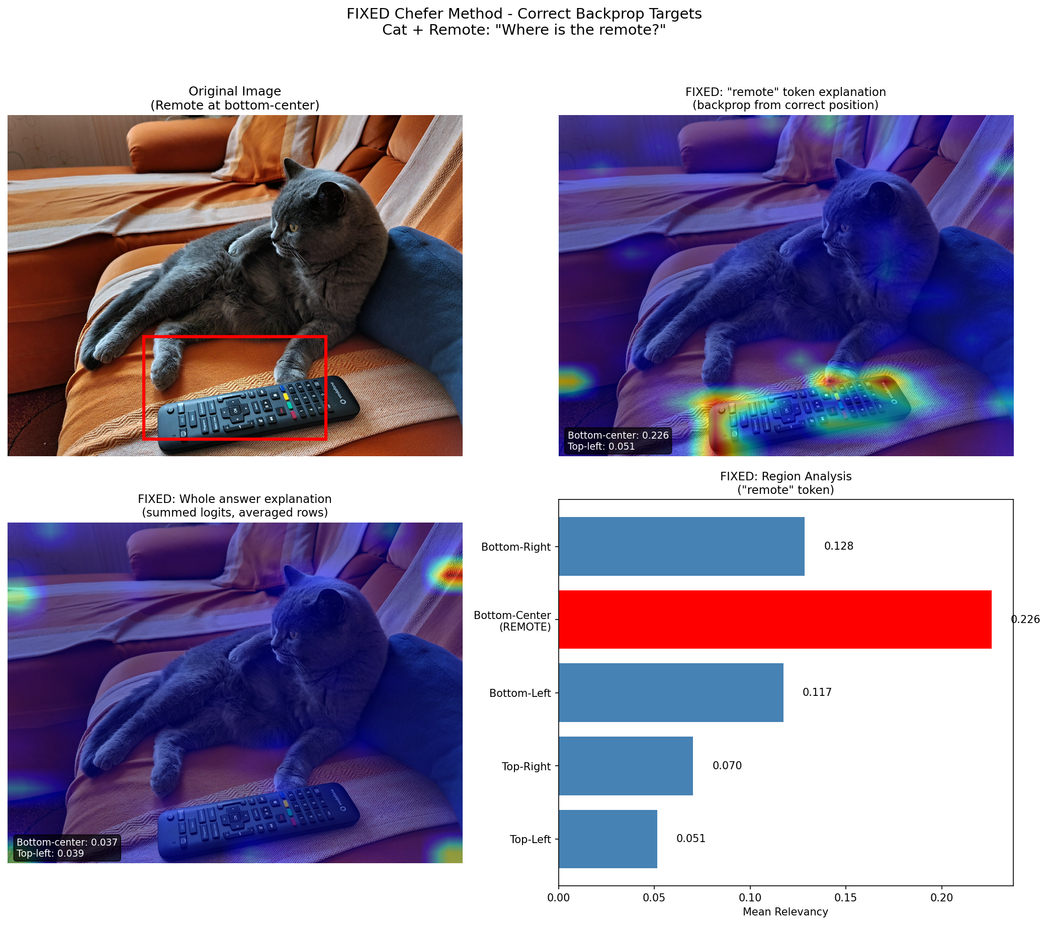
Figure 1: When explaining the “remote” token, the model’s attention is correctly focused on the bottom-center region where the remote control is located. The bar chart quantifies relevancy by region, with bottom-center scoring 0.226 compared to just 0.051 for top-left.

The bar chart on the right quantifies this. The bottom-center region (where the remote actually is) has a mean relevancy of 0.226, more than four times higher than the top-left region at 0.051. The model isn’t just producing a vague, diffuse attention pattern. It’s looking at exactly the right place.

This is the kind of sanity check that builds confidence. If the method highlighted the cat instead of the remote when explaining the word “remote,” we’d know something was wrong with either the model or our explainability implementation.

Example 2: Chest X-ray Pneumonia Detection

Now for a clinically meaningful example. Here’s a chest X-ray from a patient with right middle lobe pneumonia. A critical detail to understand: in a standard PA (posterior-anterior) chest X-ray, the image is oriented as if you’re facing the patient. This means the left side of the image corresponds to the patient’s RIGHT side.

When I ask MedGemma “Is there evidence of pneumonia?” the model generates a response mentioning consolidation in the right lung. Using the Chefer method, I can explain individual tokens in that response.

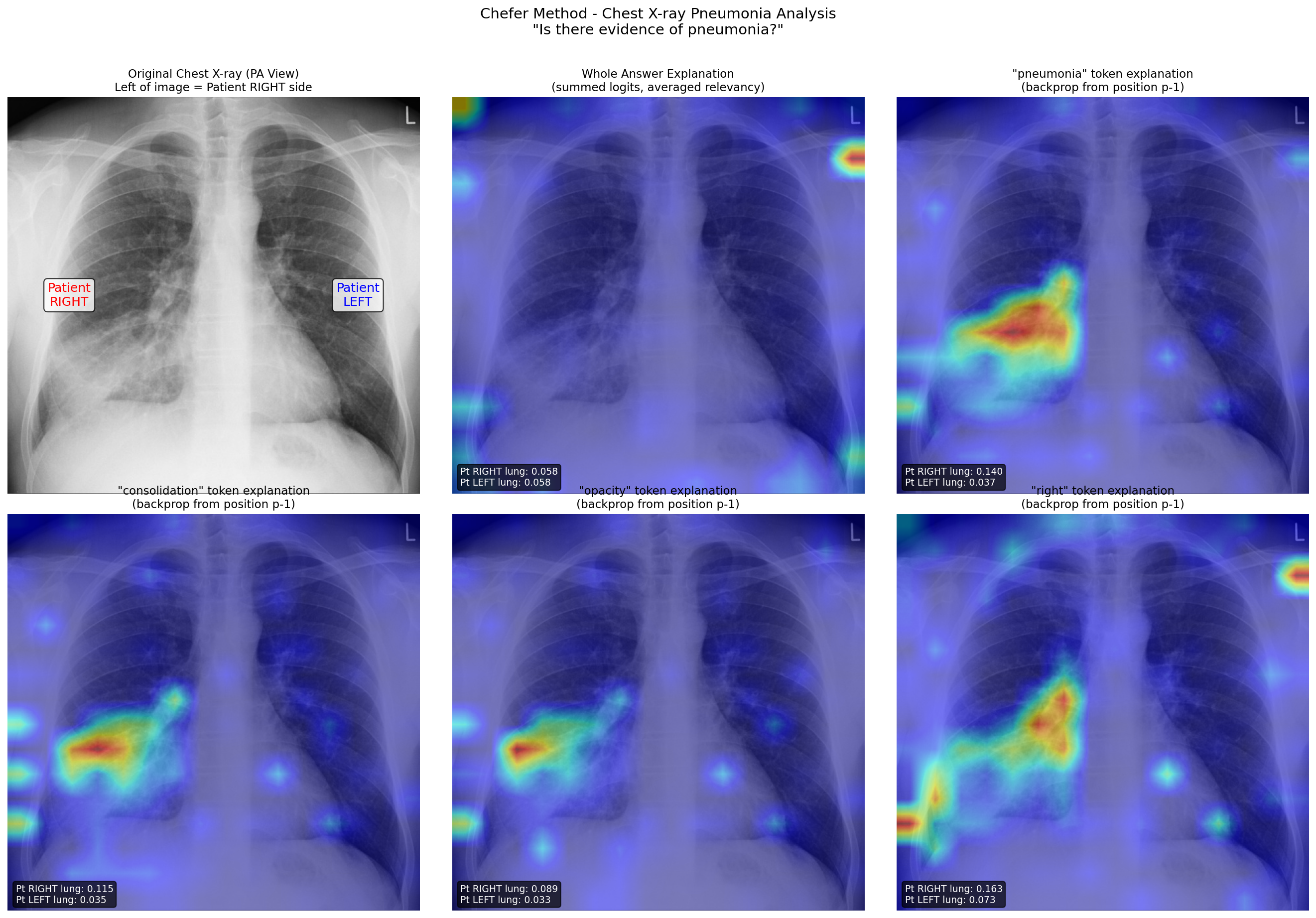
Figure 2: Chest X-ray analysis showing token-specific explanations. Top row: original image (with anatomical labels), whole answer explanation, and “pneumonia” token explanation. Bottom row: “consolidation”, “opacity”, and “right” token explanations. Each shows attention correctly focused on the patient’s right lung (left side of image) where the pathology is located.

Look at the “pneumonia” token explanation (top right). The relevancy map shows concentrated attention on the left side of the image, which is the patient’s right lung, exactly where the pathology is located. The quantitative scores confirm this: patient right lung relevancy is 0.140, nearly four times higher than the patient left lung at 0.037.

Even more striking is the “right” token explanation (bottom right of the figure). When the model generates the word “right” (as in “right lung”), the attention is strongly focused on the patient’s anatomical right side. The model isn’t just pattern-matching words; it’s correctly grounding the anatomical term to the corresponding image region.

The “consolidation” and “opacity” tokens show similar patterns, highlighting the area of increased density that characterizes pneumonic infiltration.

Part 7: A Critical Implementation Detail

While implementing this method, I discovered a subtle but crucial detail that isn’t obvious from the original paper. Getting this wrong produces meaningless results. Getting it right makes everything work.

The Backpropagation Target Problem

In causal language models like MedGemma, the logit at position i predicts the token at position i+1. This offset matters enormously for explainability.

If you want to explain why the model generated a specific token at position p, you must backpropagate from the logit at position p-1, not position p. And you should use the actual token ID that was generated, not the argmax of the logits.

Here’s the wrong approach that I see in many implementations:

# WRONG - This explains "what comes after the last token"
target_logit = logits[0, -1, logits[0, -1].argmax()]

Here’s the correct approach:

# CORRECT - This explains why the token at position p was generated
logit_position = target_token_position - 1
target_token_id = input_ids[0, target_token_position]  # The actual token
target_logit = logits[0, logit_position, target_token_id]

This distinction might seem pedantic, but it’s the difference between coherent, focused explanations and noisy, meaningless heatmaps. When I fixed this in my implementation, the results went from confusing to crisp.

MedGemma’s Architecture

For those interested in the technical details, MedGemma 1.5 4B has some architectural features that required careful handling.

The model uses 34 transformer layers with grouped-query attention, where 8 query heads share 4 key-value heads. It also employs a 5:1 ratio of local to global attention layers, where local layers only attend within a 1024-token window. Global attention layers (at positions 5, 11, 17, 23, and 29) can attend to the full sequence.

Images are processed by a SigLIP vision encoder that produces 256 image tokens arranged in a 16×16 grid. These tokens occupy positions 6 through 261 in the input sequence, with text tokens following after.

Understanding this token structure is essential for correctly extracting and visualizing image relevancy. When you pull out the first 256 values from the relevancy vector and reshape them into a 16×16 grid, you get a spatial map that can be overlaid on the original image.

Other Implementation Notes

A few other details that matter:

Use eager attention: MedGemma’s default SDPA (Scaled Dot Product Attention) implementation doesn’t support output_attentions=True. You need to load the model with attn_implementation="eager".
Keep the model in eval mode: Use torch.enable_grad() context instead of calling model.train(). This preserves the inference behavior while allowing gradient computation.
Convert to float32: Attention tensors come out as bfloat16. Convert them to float32 for stable gradient computation.
Retain gradients: Call attn.requires_grad_(True) and attn.retain_grad() on the attention tensors before the backward pass.

Part 8: Implications for Medical AI Safety

Let me return to where we started: the challenge of trusting AI in medicine.

Medical decisions carry enormous stakes. A false negative might mean a missed cancer. A false positive might mean unnecessary surgery. We can’t simply trust AI systems because they score well on benchmarks. We need to verify they’re reasoning correctly.

The Chefer method gives us a tool for this verification. When a model says “this X-ray shows signs of pneumonia,” we can ask “show me what you’re looking at.” If the heatmap highlights the lung region with the suspicious opacity, our confidence increases. If it highlights the patient’s ID number or the machine manufacturer’s logo, we know something is wrong.

This isn’t just about catching errors. It’s about building appropriate trust. Explainability lets us calibrate our reliance on AI to match its actual capabilities. We might trust the model more in situations where its attention patterns look sensible, and trust it less when its reasoning seems confused.

The Limitation to Remember

One important caveat: attention-based explanations show us what the model looked at, not necessarily why. Two models might look at the same region but interpret it differently. One might correctly identify an abnormality, while another might misclassify it.

Think of it this way: if two doctors are examining the same X-ray, knowing they’re both looking at the lower right lung is useful, but it doesn’t guarantee they’ll reach the same conclusion. The attention map is the “where,” not the “what” or “why.”

This means explainability methods are one tool among many. They’re most powerful when combined with other approaches like testing on diverse datasets, comparing to expert annotations, and conducting systematic error analysis.

Conclusion: Opening Doors, Not Just Black Boxes

We’ve covered a lot of ground in this post. We started with the problem of understanding what AI models are looking at, built up an understanding of how attention works in transformers, and walked through a method that traces relevance through multi-layer networks.

The Chefer method is elegant because it respects the actual computational structure of transformer models. Rather than treating the network as an inscrutable black box, it uses the model’s own attention patterns and gradients to surface meaningful explanations.

For those working with medical AI, methods like this are essential. They transform the question “can we trust this model?” from philosophical hand-wraving into concrete investigation. We can look at what the model sees, compare it to clinical expectations, and make informed decisions about deployment.

Try It Yourself

The complete implementation is available on GitHub:

github.com/thedatasense/medgemma-explainer

The repository includes:

Full source code for the explainability method
Jupyter notebook tutorials
Example scripts for medical image analysis
Visualization utilities

Feel free to use it, extend it, and let me know what you discover.