I’ve been focused on a problem for months. I feed a chest X-ray into a Vision-Language Model (VLM) and ask: “Is there evidence of cardiomegaly?” The model says yes, with reasonable confidence. Then I ask the exact same model, looking at the exact same image: “Can you rule out cardiomegaly?” And it says yes to that too.
Same image. Same visual attention map. Completely opposite diagnostic conclusions. I started calling this the “flip-with-stable-focus” phenomenon, and it kept me up at night (It still keeps me up). How could a model that’s clearly looking at the right anatomical region still flip its answer based on how I phrased the question?
Edward Lorenz and the butterfly that broke everything
Edward Lorenz was a meteorologist at MIT trying to model weather patterns with a simple system of three differential equations. One day in 1963, he restarted a simulation but rounded one of his input values from 0.506127 to 0.506. That tiny difference, smaller than a rounding error, produced a completely different weather forecast after a few simulated days.
This is the Butterfly Effect, and Lorenz formalized it through what we now call the Lorenz system: a set of three coupled ordinary differential equations that produce chaotic trajectories from nearly identical starting points. There is a very interesting to explore simulator here.
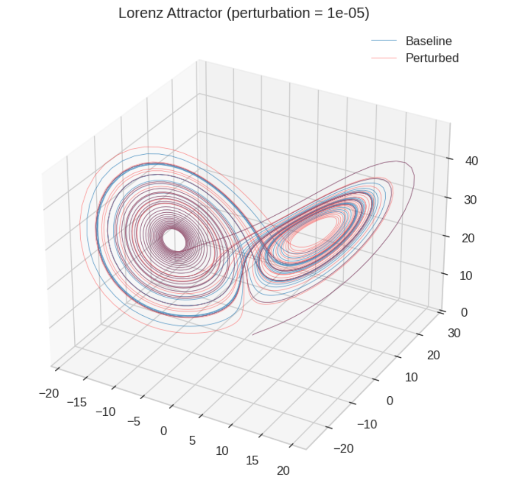
I ran the classic simulation myself. Two trajectories start at initial conditions separated by just 0.00001 in the x-coordinate. For a while, they track each other perfectly. You’d think they were the same system. Then, suddenly, they diverge and end up on completely different wings of the attractor.
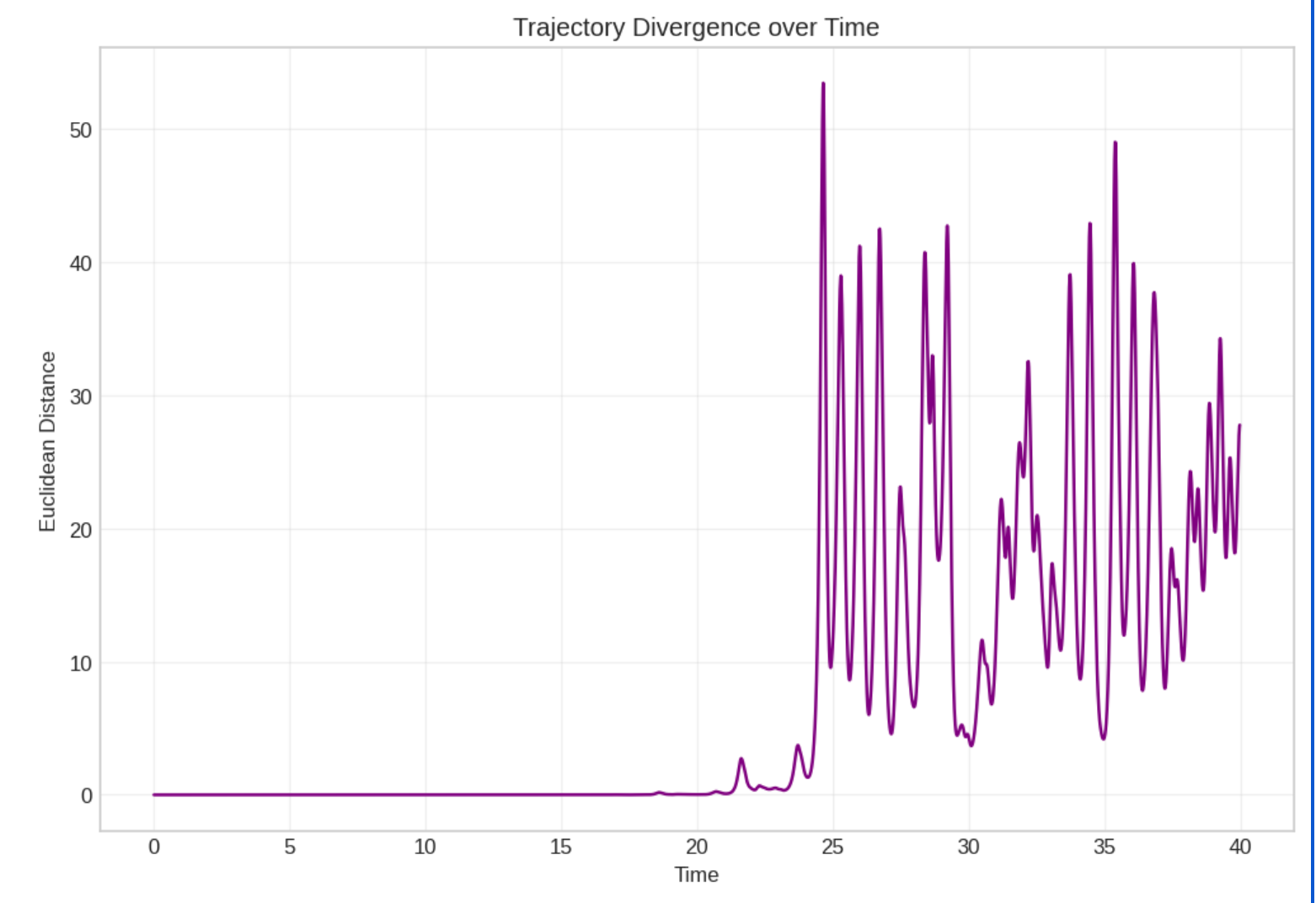
The divergence plot is what caught my eye. The distance between the two trajectories stays near zero for a long stretch (local stability), then suddenly explodes upward. That shape looked very familiar. It looked like what happens inside a neural network when you perturb the input just slightly.
Want to run this yourself? I’ve put together a Colab notebook where you can reproduce the Lorenz simulation, the network dynamics experiment, and the Lyapunov estimation. Everything is set up for parameter sweeps so you can explore the space on your own.
Neural networks are dynamical systems
Here’s the connection that changed my thinking. A deep neural network, whether it’s a ResNet or a Transformer, is a discrete dynamical system. Each layer takes an activation vector and transforms it:
$$\mathbf{x}_{t+1} = f(\mathbf{W}_t \cdot \mathbf{x}_t)$$Layer index (t) is like time. The activation (\mathbf{x}_t) is like the state of the atmosphere. The weight matrix (\mathbf{W}_t) determines whether perturbations grow or shrink as they propagate through depth.
The critical quantity is the spectral radius of the weight matrix: the magnitude of its largest eigenvalue.
| Spectral Radius | Behavior | Neural Network Effect |
|---|---|---|
| < 1.0 | Ordered | Perturbations shrink. Gradients vanish. Network forgets input details. |
| ≈ 1.0 | Edge of Chaos | Balance between sensitivity and stability. Best for learning. |
| > 1.0 | Chaotic | Perturbations explode. Gradients blow up. Tiny input noise becomes catastrophic. |
I simulated this directly. I created a 100-dimensional recurrent system with tanh nonlinearities (a stripped-down proxy for a deep network) and fed it two inputs that differed by (10^{-5}). With spectral radius 0.9, the perturbation decays through the layers. The network is stable, maybe too stable. With spectral radius 1.5, the perturbation grows exponentially. By layer 30, the two outputs have nothing in common.
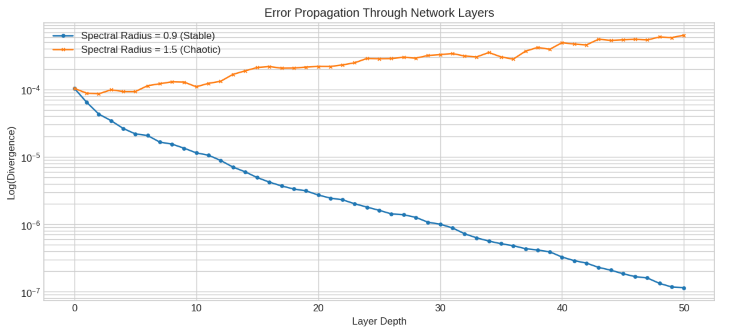
That exponential divergence is exactly what I see in my VLM experiments when a rephrased question causes a diagnostic flip.
Measuring instability with a number: the Lyapunov exponent
Physicists have a precise tool for quantifying chaos. The Lyapunov exponent ((\lambda)) measures how fast nearby trajectories separate:
$$\lambda = \lim_{t \to \infty} \frac{1}{t} \ln \frac{\| \delta(t) \|}{\| \delta(0) \|}$$If (\lambda) is positive, the system is chaotic. Perturbations grow. If negative, it’s stable. Perturbations shrink. If approximately zero, the system sits at the edge of chaos.
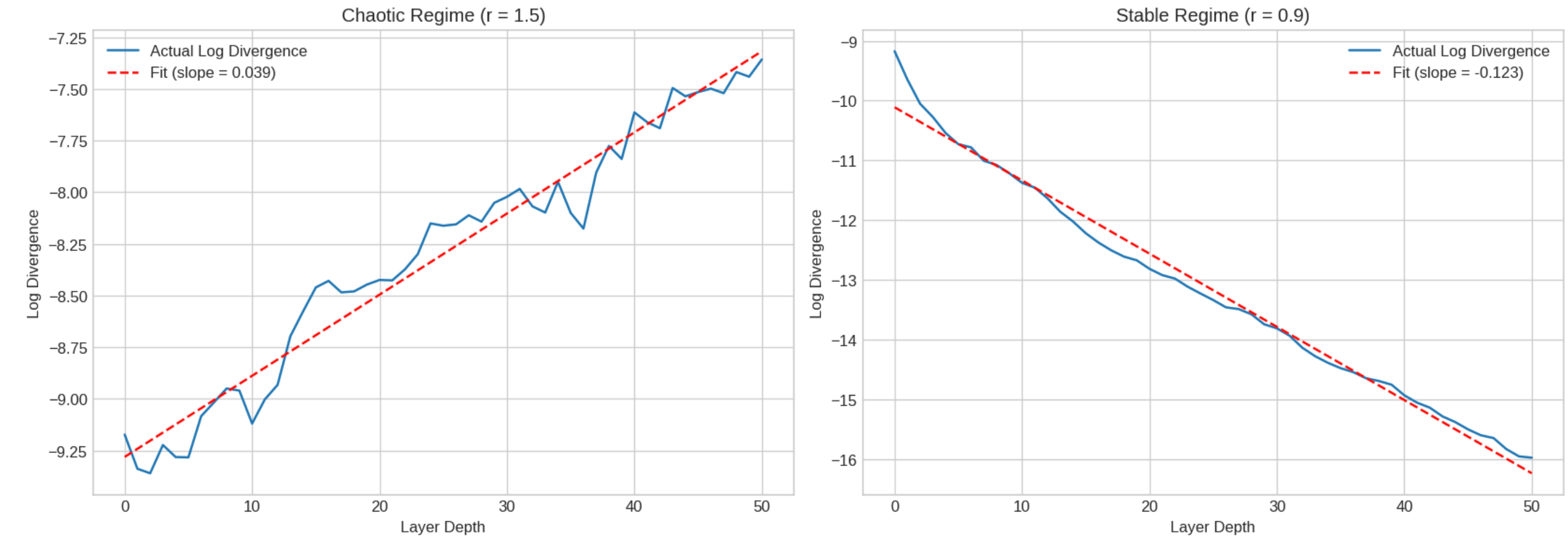 This is just the slope of the log-divergence curve, which makes it easy to compute from simulation data. Feed two slightly different inputs through your network, measure the Euclidean distance between activations at each layer, take the log, fit a line. The slope is your Lyapunov exponent.
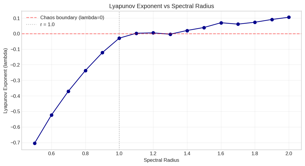
I swept spectral radius from 0.5 to 2.0 and computed (\lambda) at each value. The resulting curve crosses zero right around spectral radius 1.0, exactly where theory predicts the onset of chaos. Below 1.0, the network is a contraction mapping. Above 1.0, it’s an expansion.
So what does this mean for medical VLMs?
This is where it gets practical for my dissertation work. I’m studying models like MedGemma and LLaVA-Rad on chest radiographs from the Medical Information Mart for Intensive Care (MIMIC-CXR) dataset. The “flip-with-stable-focus” phenomenon I described at the start can be reframed in chaos theory terms.
When I rephrase a diagnostic question, I’m applying a small perturbation to the language embedding. The visual pathway stays stable (the attention map doesn’t change, hence “stable focus”). But the language pathway, or more precisely the cross-modal fusion layers, amplifies that perturbation until the output flips.
In Lyapunov terms: the visual encoder has negative (\lambda) (contractive, stable). The language-conditioned layers have positive (\lambda) (expansive, chaotic). The model as a whole is chaotic because one subsystem is chaotic, even though another is stable.
This gives me a concrete research plan:
| Step | Method |
|---|---|
| 1 | Extract per-layer activations from the VLM for paired phrasings of the same diagnostic question |
| 2 | Compute the divergence trajectory across layers |
| 3 | Estimate (\lambda) at each layer to build a “Lyapunov spectrum” of the model |
| 4 | Identify which layers cross the chaos boundary, and whether they correspond to the cross-attention or fusion layers |
If the hypothesis holds, the unstable layers should cluster around the cross-modal fusion points. That would tell us exactly where to apply regularization, spectral normalization, or architectural changes to make the model more phrasing-invariant.
The honest version of how I got here
I’ll admit this connection wasn’t obvious to me at first. I spent weeks looking at attention maps trying to understand why the model flipped, because attention visualization is what everyone does. The maps were stable. The answers weren’t. I was stuck.
The chaos theory framing clicked during a conversation about the Lorenz system that had nothing to do with my research. I was explaining the Butterfly Effect to someone, drew the divergence plot on a napkin, and realized I’d seen that exact shape in my layer-by-layer analysis of VLM activations. Sometimes the best research insights come sideways.
What I’m still figuring out
A few open questions keep me honest about how far this analogy goes.
First, real neural networks have structured weight matrices trained by gradient descent, not random matrices. The spectral properties of trained weights could behave differently than what the random matrix simulation predicts. I need to measure, not assume.
Second, the Lyapunov exponent assumes infinitesimal perturbations and infinite time. In a 32-layer Transformer, we have finite perturbations propagating through finite depth. The Finite-Time Lyapunov Exponent (FTLE) is the right tool here, but its reliability depends on the perturbation size and layer count. I’ll need to validate with multiple perturbation magnitudes.
Third, and this is the exciting part: if the Lyapunov spectrum does localize instability to specific layers, we might be able to design targeted interventions rather than applying blanket regularization. Spectral normalization on just the chaotic layers. Architectural changes at just the fusion points. That’s the practical outcome I’m working toward.
Weather forecasters learned to live with chaos by building ensemble methods and quantifying uncertainty. Medical VLMs might need to do the same thing, and the first step is knowing exactly where in the model the chaos lives.